
One Paper. One Matrix Operation. Every Vendor Alibi, Eliminated.

Welcome to the Ethics & Ink AI Newsletter #64

How DAMP actually works — and what five figures from a Johns Hopkins paper prove about AI memory, vendor accountability, and the architecture of real deletion!
Last Week, In Case You Missed It
Last issue introduced a paper that changed the frame of the fight.
Three researchers at Johns Hopkins — Hatami, Aalishah, and Monosov — published DAMP on April 16th, 2026. You can read that paper here. The short version: they built a machine unlearning method that actually works. As I understand it, one matrix operation. No training loop. No backpropagation. Runs in seconds. And unlike every other commercial method on the market, it removes data’s influence at the representational level — not just at the output.
Most vendors have been selling you logit masking — a trick where the model stops saying your name while still knowing everything about you. The internal features that identify you stay fully intact, fully decodable, sitting right there in the deep layers waiting for anyone with audit authority to find them. DAMP produces forgetting that survives that audit. The competition does not.
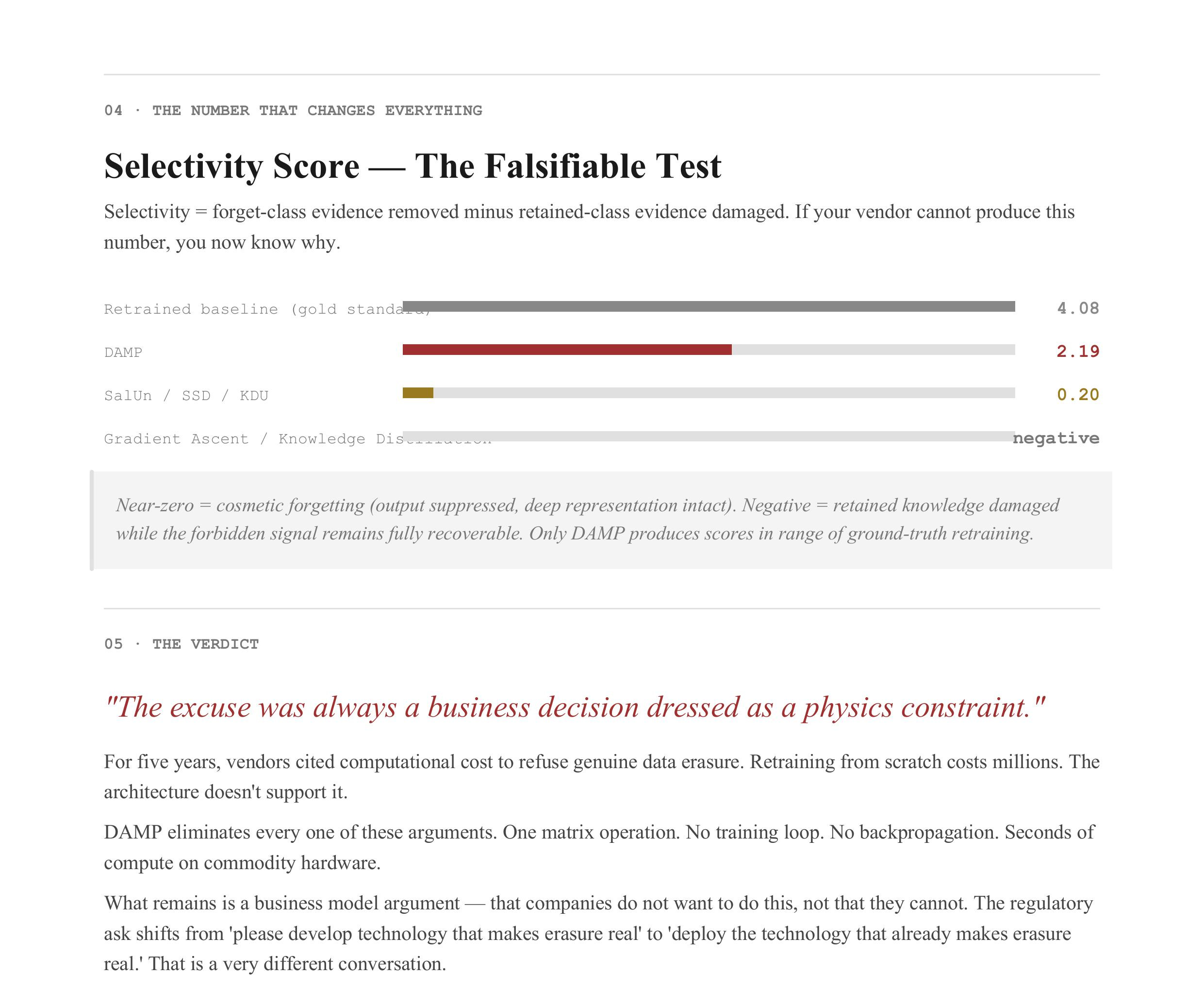
The selectivity metric — a measurement of how much forbidden evidence was actually removed minus how much retained evidence was damaged — put a number on it: 4.08 for a fully retrained model (the gold standard), 2.19 for DAMP, and near-zero or negative for the entire vendor catalog. Near-zero means they barely forgot anything. Negative means they broke the retained knowledge while leaving the forbidden signal recoverable. DAMP is the only approximate method in striking distance of ground truth.
That was last week. The claim was made. Today, we look at the proof. But first — the machine itself.
How a Neural Network Actually Works
You cannot understand what DAMP is doing to a model without understanding what a model is. So here’s the honest version — no hype, no hand-waving.
A neural network is, at its core, a very large function. You put something in — an image, a sentence, a medical record — and it produces a prediction. What happens in between is the part that most vendors are counting on you to just accept as your “AI black box.”
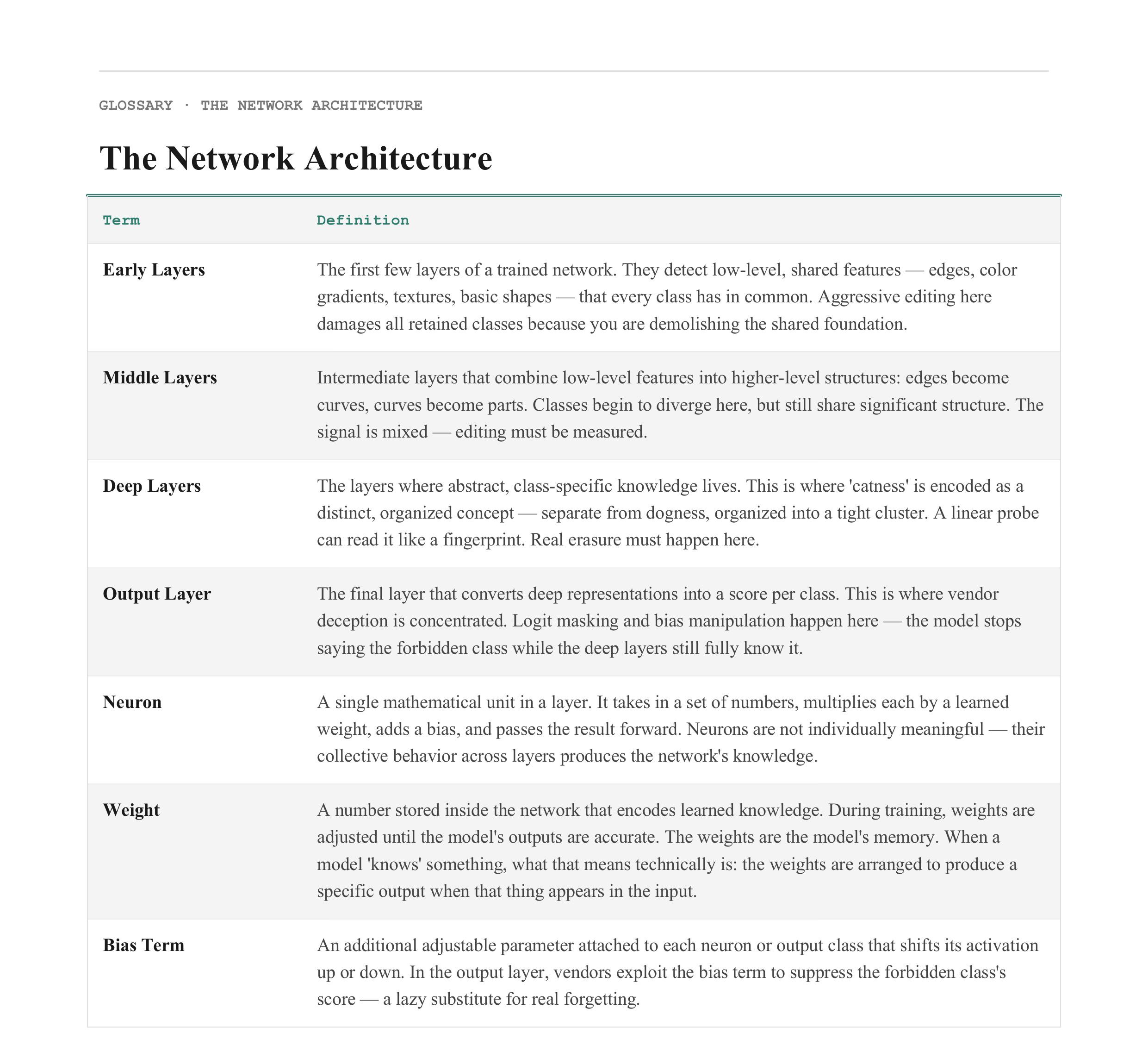
To exactly, this network is organized in layers. Each layer is a collection of neurons — mathematical units that take in a set of numbers, multiply them by a set of weights, add a bias term, and pass the result forward. The weights are the network’s memory. They encode everything the model learned during training. When you hear that a model “knows” something, what that means technically is: the memory is arranged in a way that produces a specific output when that thing appears in the input.
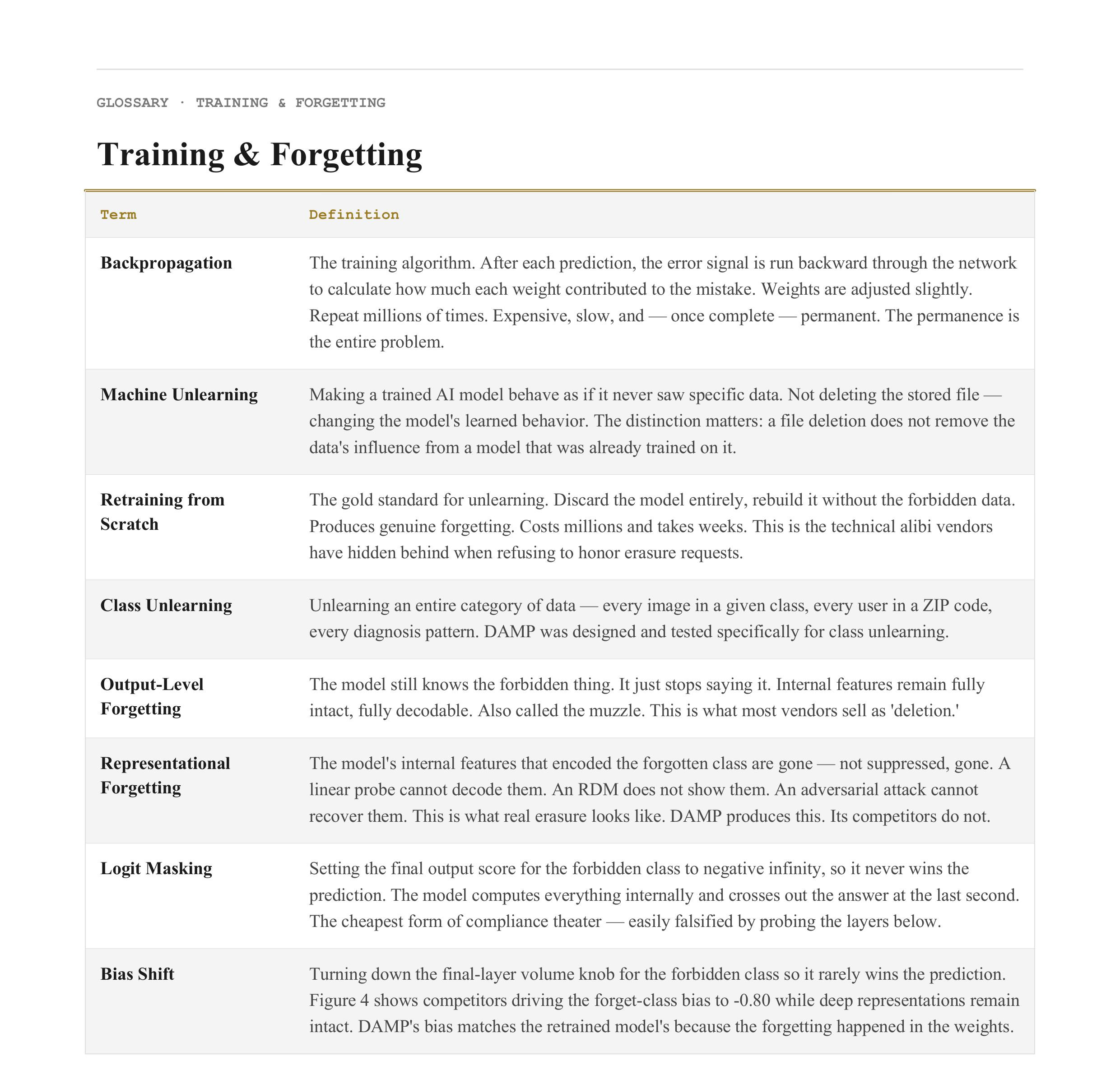
Training is the process of adjusting those memories until the model’s outputs are accurate. You show the model a million cat photos labeled “cat,” adjust the weights a tiny amount each time the model gets it wrong, and repeat until it gets it right. The process is called backpropagation — you run the error signal backward through the network to figure out how much each weight contributed to the mistake, and you nudge accordingly. This process is expensive. It requires enormous amounts of compute and memory. It is also, once done, permanent— which is the entire problem.
What Happens at Each Layer
Here is where the “depth-aware” part of DAMP’s name earns its meaning.
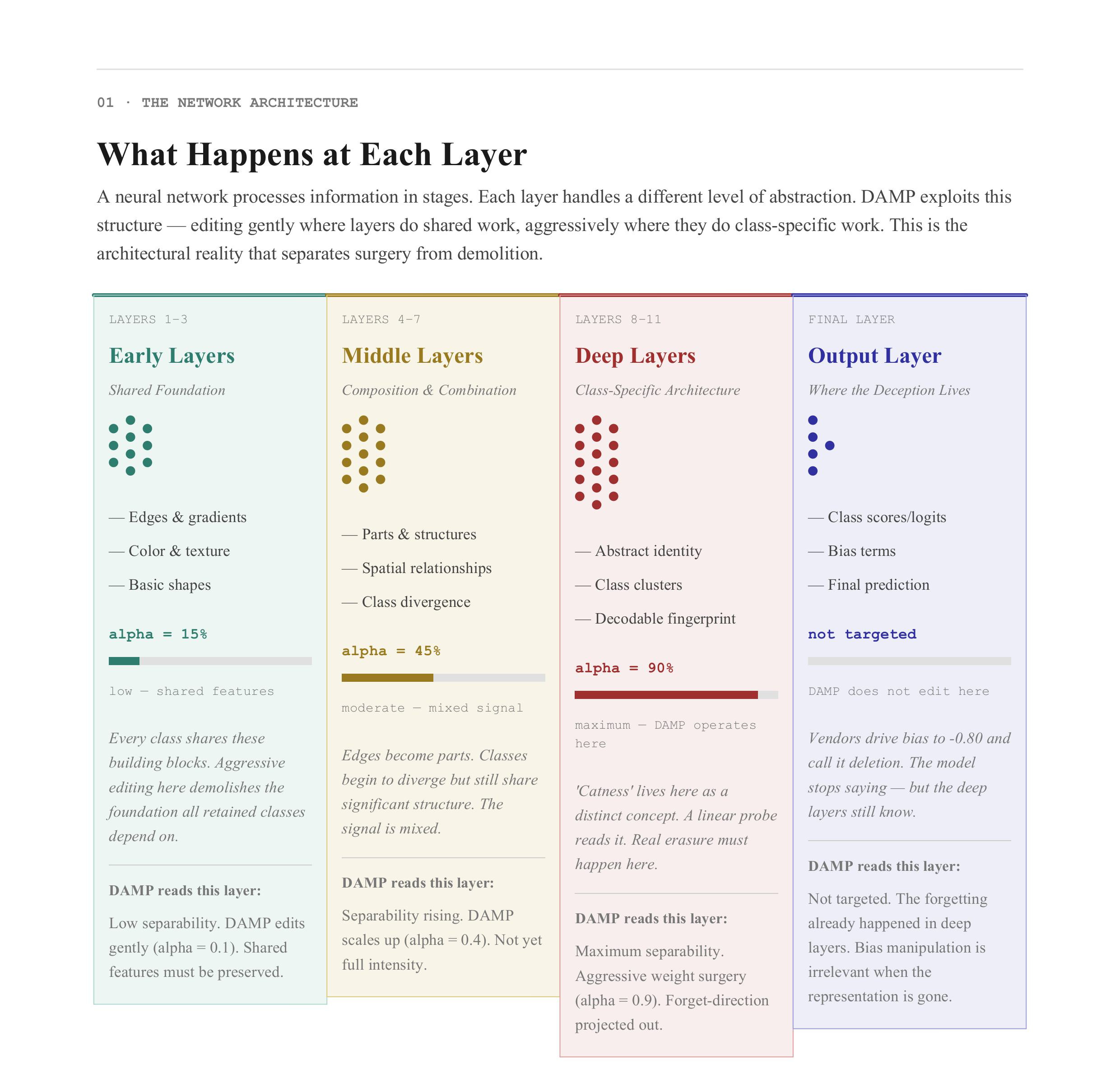
Not all layers do the same thing. A neural network processes information in stages, and each stage handles a different level of abstraction. This is one of the most well-documented and reproducible findings in machine learning research, and it is the architectural reality DAMP exploits.
Early layers: the shared foundation. The first few layers of a trained network detect low-level features: edges, color gradients, textures, simple shapes. A cat and a dog and a car all have edges. They all have textures. The early layers are doing shared work that every class depends on. If you aggressively edit early-layer weights, you damage the foundation that all retained classes are built on. You’re not performing surgery — you’re demolishing the building.
Middle layers: composition and combination. The middle layers begin combining low-level features into higher-level structures. Edges become curves. Curves become shapes. Shapes become parts — an ear, a wheel, a corner. At this stage, a cat and a dog are starting to diverge, but they still share significant structure (four legs, bilateral symmetry, similar scale). The signal is mixed. A method that edits these layers without accounting for what is shared and what is class-specific will produce collateral damage.
Deep layers: the class-specific architecture. The deep layers are where the abstract class representation lives. This is the layer that encodes “catness” as a distinct, recognizable concept — separate from dogness, separate from birdness, organized into a tight cluster in the high-dimensional space the network operates in. This is the layer a linear probe can read like a fingerprint. This is the layer where a model that claims to have forgotten cats but hasn’t can be caught. The deep layers are where real erasure has to happen.
The output layer: where the deception lives. The final layer takes the deep representation and converts it into a score for each possible class. This is where logit masking operates. This is where bias manipulation happens. A vendor can suppress your class at this layer while leaving everything in the layers below it completely intact. Figure 4 shows exactly this: competitors cranking the final-layer bias for the forgotten class down to −0.80. The model still knows. It just stops saying.
This layered architecture is not a quirk of one specific model. It is a property of deep neural networks generally, replicated across architectures, replicated across tasks, replicated across the benchmarks in the DAMP paper: a small CNN, ResNet-18, and a Vision Transformer. The depth structure holds.
DAMP works because it takes this structure seriously. Every other method on the market treats the network as a uniform object to be optimized. DAMP treats it as a layered architecture to be read and edited precisely.
This Week’s Vocabulary
With the architecture in view — here are some additional terms you’ll need for the figures:
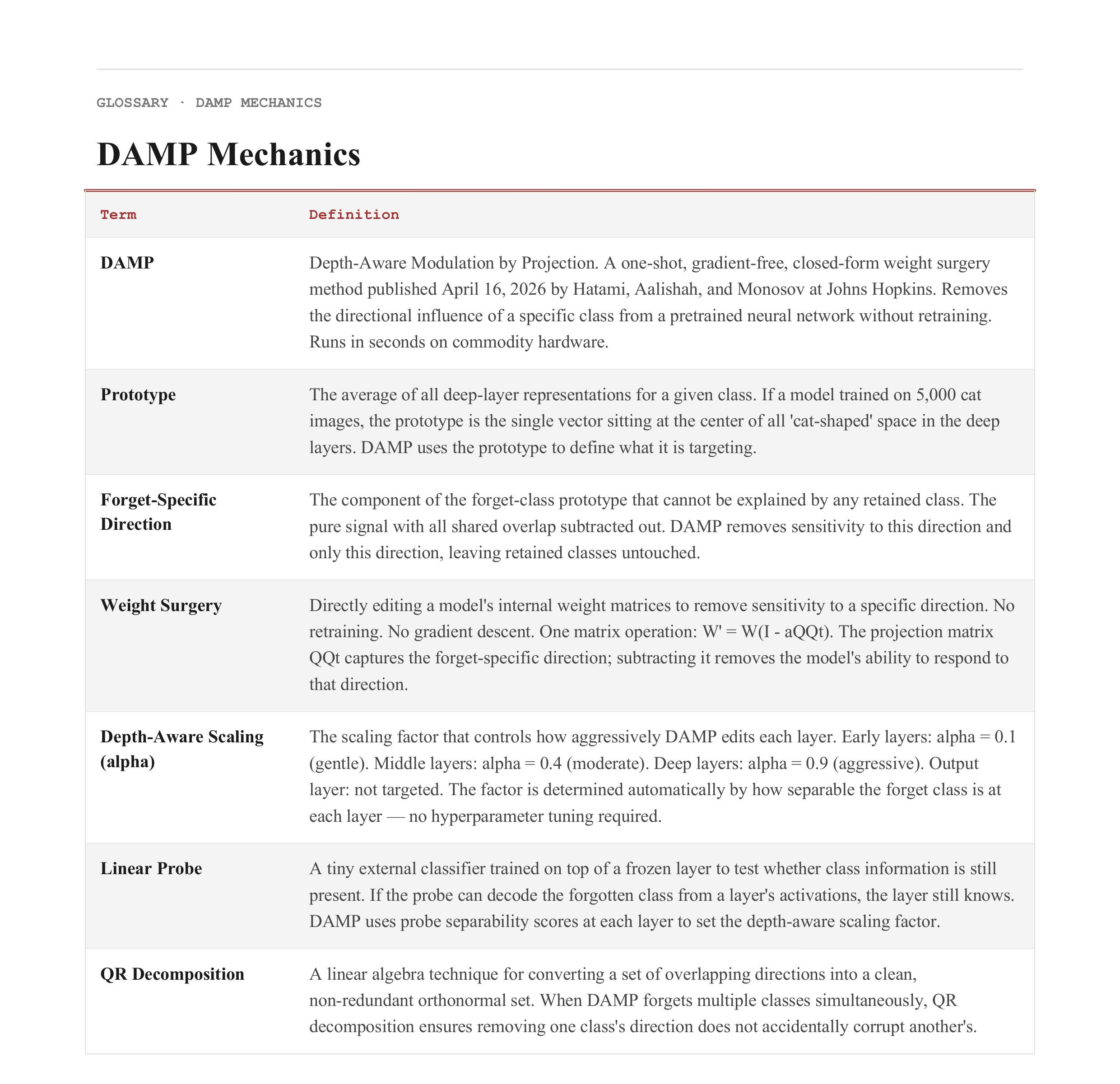
(1) Prototype — The average of all the deep-layer representations for a given class. If a model has seen 5,000 cat images, the prototype is a single vector sitting at the center of all the “cat-shaped” space in the deep layers. DAMP uses this to define what it’s targeting.
(2) Forget-specific direction — The component of the forget-class prototype that cannot be explained by any other class. This is the pure cat-signal, with all shared mammal-texture-furry-creature overlap subtracted out. DAMP targets this and only this.
(3) Weight surgery — Directly editing a model’s internal weight matrices to remove sensitivity to a specific direction. No retraining, no gradient descent. One matrix operation: W′ = W(I − αQQᵀ).
(4) Depth-aware scaling — The insight that early layers should be edited gently (shared features) and deep layers aggressively (class-specific features). The scaling factor sets itself based on how separable the forget class is at each layer. No hyperparameter tuning required.
(5) Linear probe — A tiny external classifier trained on top of a frozen layer to test whether class information is still there. If the probe can decode the forgotten class from that layer’s activations, the layer still knows. DAMP uses probe separability to calibrate depth scaling.
(6) RDM (Representational Dissimilarity Matrix)— A map of how different classes appear to a given layer from the inside. After real unlearning, the forgotten class should dissolve — lose its distinct cluster, stop having a coherent neighborhood.
(7) QR decomposition — A linear algebra technique for turning overlapping directions into a clean, non-redundant set. DAMP uses this when forgetting multiple classes simultaneously to ensure removing one class’s direction doesn’t corrupt another’s.
(8) VRAM — GPU memory. Retraining a large model can require 40–80GB and take days. DAMP’s one-pass approach uses a fraction of that.
The Five Figures
With the architecture understood and the vocabulary in hand, here is what the paper actually proves.
Figure 1 — Why DAMP Is the Only Method That Scales
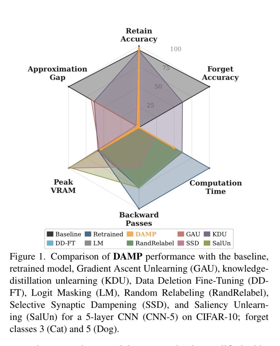
Figure 1 is the efficiency comparison, and it is not close.
It plots computation time and VRAM usage for every method tested. DAMP sits at the bottom-left corner of both: least time, least memory. Competitors cluster at the top-right. The gap is not marginal. It is architectural.
This is the direct result of DAMP’s one-shot design. Every other method runs an iterative optimization loop — hundreds or thousands of passes through the model, computing gradients, adjusting weights, checking results, repeating. Gradient Ascent alone can require thousands of iterations before forget-accuracy drops to an acceptable level. DAMP computes the forget-specific direction once, applies the projection once, and stops. No backprop. No training loop.
The cost argument — “true erasure requires retraining from scratch, and retraining is economically prohibitive” — has been the industry’s most durable stall for five years. Figure 1 is the direct technical refutation. The method exists. It runs on commodity hardware. It takes seconds. The cost argument is now a business preference dressed as a physics constraint.
There is no longer a compute excuse. There is only a compliance choice.
Figure 2 — The Selectivity Score: Putting a Number on the Lie
Figure 2 is the one you hand to a regulator.
Selectivity is defined as how much forget-class evidence was actually removed, minus how much retained-class evidence was damaged in the process. A perfect score would mean complete forgetting with zero collateral damage. The retrained baseline — rebuild the model from scratch without the forbidden data — scores 4.08. DAMP scores 2.19. Every other method scores near-zero or negative.
Near-zero means the method gamed the output metric while leaving the representation intact. It suppressed the final-layer bias and called it deletion. The RDM still shows the forgotten class. The linear probe can still decode it. The forgetting is cosmetic.
Negative means the method degraded the retained classes — damaged the architecture’s shared foundations in the early and middle layers, as described above — while still failing to remove the forgotten class from the deep layers where it actually lives. It broke the building while leaving the crime scene intact. The worst possible outcome.
What Figure 2 gives you is a falsifiable, reproducible test. You can apply this metric to any vendor’s claimed implementation. If they cannot produce a selectivity score, or if their score is near-zero, you now know precisely what their compliance is worth. This is the forensic instrument Law 7 enforcement has been waiting for: not a policy argument, not a moral claim, a number. A number that can go in a compliance order.
Figure 3 — The Geometry of Genuine Forgetting
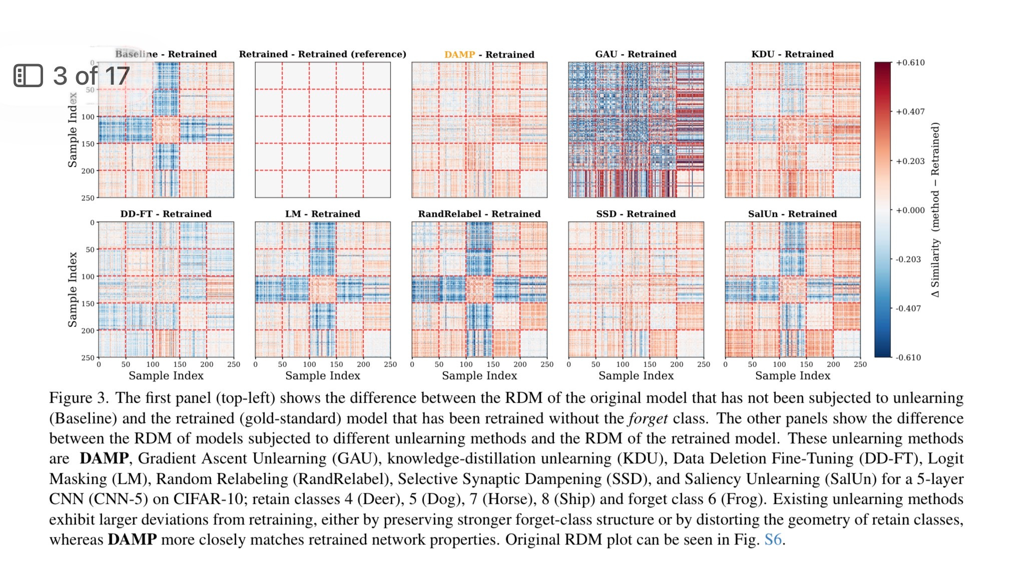
Figure 3 is the proof that DAMP’s forgetting reaches the interior of the architecture.
A Representational Dissimilarity Matrix is a snapshot of how a network’s internal layers organize knowledge. Every class gets plotted relative to every other class based on how similar their internal activations are in the deep layers. Classes the network treats as related sit close. Classes it treats as distinct sit far apart. The RDM is a map of the model’s internal world — how it has carved up the space of everything it learned.
After genuine unlearning, the forgotten class should dissolve on this map. Its internal representation should become indistinguishable from noise. It should stop having a coherent neighborhood — the tight cluster of deep-layer activations that a linear probe can decode, that an adversarial attack can exploit, that a subsequent fine-tuner can resurrect.
DAMP’s RDM after forgetting closely matches the retrained model’s RDM. The forgotten class is gone from the internal geometry. The competitors’ RDMs do not match. Even when a competing method successfully drives forget-accuracy to zero at the output layer, the deep-layer geometry remains organized around the forgotten class. The map still shows it. The probe can still find it.
Figure 3 is the X-ray that shows what is hiding behind the muzzle. It is the difference between a compliance claim that survives forensic scrutiny and one that doesn’t.
Figure 4 — The Bias Trick, Exposed
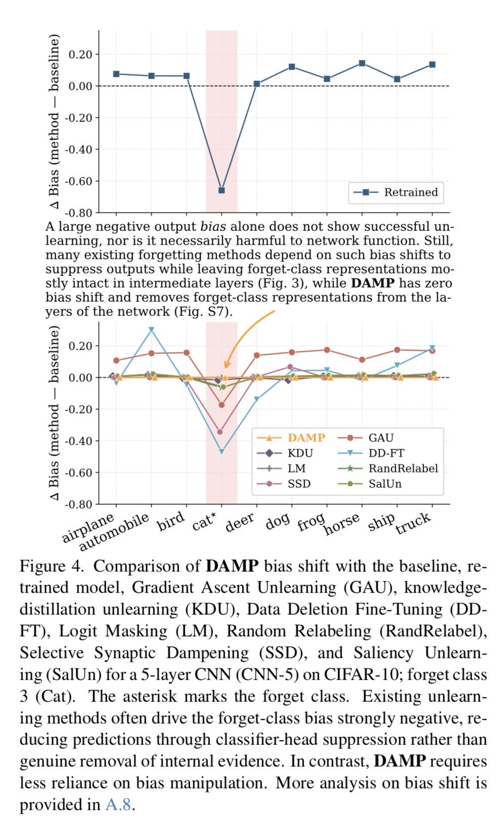
Figure 4 is where the mechanism of the fraud becomes visible at the layer level.
In a classification model, the output layer assigns a score to each class before a prediction is produced. That score is shaped in part by a bias term — a volume knob that makes a given class more or less likely to win. One of the most common forms of fake unlearning is simply cranking that bias for the forbidden class down to a very large negative number. The deep layers still carry the full class representation. The middle layers still encode the class-specific composition. But the output layer is muzzled, so the model never says the forbidden word.
Figure 4 plots the forget-class bias for every method tested. Competitors cluster hard around −0.80 or lower. They are all, to varying degrees, executing the same final-layer trick. Bias manipulation. Output suppression. The muzzle.
DAMP’s forget-class bias after unlearning matches the retrained model’s bias. It does not rely on the trick. And the supplemental experiment confirms exactly why: when the researchers forced DAMP’s output bias to match a competitor’s −0.80 value, nothing changed. Retain accuracy held at 92.4%. Forget accuracy stayed at 0%. The forgetting was already done by the weight surgery in the deep layers. The output-layer bias was irrelevant because the representation was already gone.
Figure 4 is not just a benchmark result. It is a taxonomy of the industry’s preferred deception strategy, laid out layer by layer in a bar chart with error bars. The fraud lives at the output layer. The evidence lives everywhere else.
Figure 5 — Why Depth Awareness Is the Whole Game
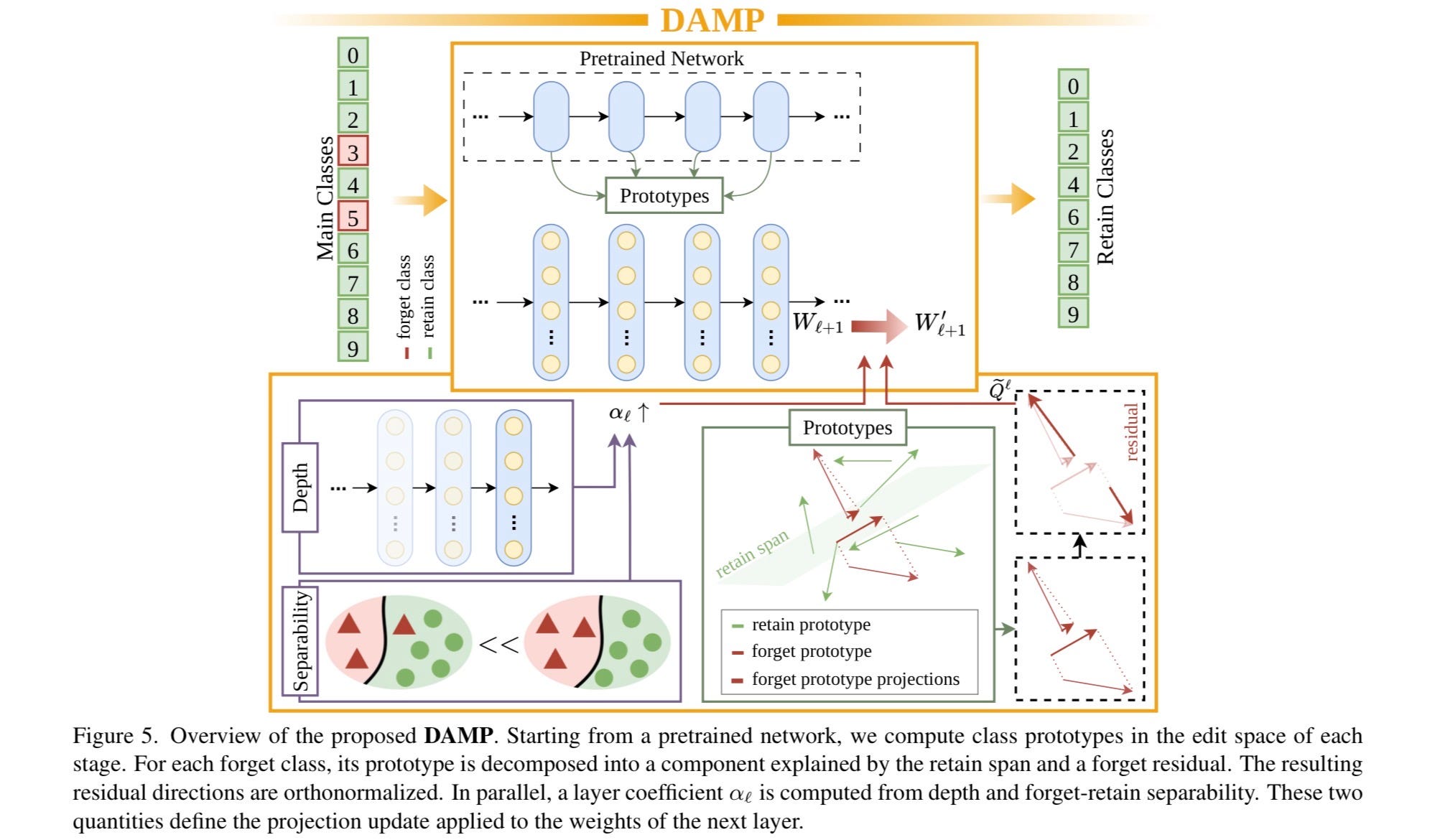
Figure 5 is the paper’s argument for its own central design choice — and the most important figure for understanding why DAMP outperforms methods that also claim to do weight editing.
The “D” in DAMP stands for depth-aware. Figure 5 shows the scaling factor α plotted across network depth, separately for the forget class and the retain classes. It is a direct visualization of the layer-by-layer architecture described above: in early layers, the forget and retain classes are not easily separable — the layer is doing shared work, and the scaling factor is low. In deep layers, the forget class becomes linearly separable from the retain classes — the layer is doing class-specific work — and the scaling factor rises. The edit becomes more aggressive precisely where it must be and gentler precisely where it would cause damage.
This is the self-calibrating mechanism. The network tells DAMP how hard to edit each layer. The formula reads the model’s own separability structure at each depth using a linear probe, and responds accordingly. No hyperparameter tuning. No human guessing at the right balance between forget-accuracy and retain-accuracy. The architecture provides the answer.
Competitors that do not account for depth divide into two failure modes, both visible in Figure 2’s selectivity scores. Under-edit: apply a uniform weak projection everywhere, and the deep layers retain the class-specific representation intact. Over-edit: apply a uniform aggressive projection everywhere, and the early layers’ shared foundations get destroyed along with the forgotten class. Both failures show up in the data. Both are architectural errors traceable to the same root cause: treating the network as a uniform object when it is not.
DAMP threads the needle because it reads the architecture before it edits it. That is the depth-awareness. That is why it works.
Next Issue
Next week is the one built for a specific Tuesday morning meeting with a specific vendor.
We turn these five figures into a procurement toolkit. The audit questions. The contract language. The exact regulatory ask that a GDPR and EU AI ACT enforcement body can operationalize and that a vendor cannot dismiss as technically unreasonable — because this paper just closed that exit.
The compliance theater had a technical alibi. The technical alibi is now evidence in the opposite direction. Next issue: exactly how we use it.
— Chara

Founder, The Praesidium Institute
Author, The 10 Laws of AI: A Battle Plan for Human Dignity in the Digital Age
Publisher, Ethics & Ink — AI
P.S. — The selectivity score is a falsifiable test. If your vendor can’t produce one, that’s the answer.
P.P.S. — DAMP’s depth-awareness is not a complexity feature. It is a precision feature. Surgery, not demolition. The distinction matters every time someone’s data is in the model.
P.P.P.S. — Hatami, Aalishah, Monosov. Johns Hopkins. April 16, 2026. Free to read. Put it in your vendor meeting agenda before they do.